Joint inversion of surface-wave dispersion and receiver function

import bayesbay as bb
from bayesbay.discretization import Voronoi1D

from functools import partial
import string
import numpy as np
import matplotlib.pyplot as plt
import matplotlib.gridspec as gridspec
from matplotlib.ticker import MaxNLocator, AutoLocator, FixedLocator
from disba import PhaseDispersion # install disba for forward modelling of dispersion curves
import pyhk  # Install pyhk for forward modelling of receiver functions 

np.random.seed(30)
np.seterr(all="ignore");

THICKNESS = np.array([10, 10, 15, 20, 20, 20, 20, 20, 0])
VS = np.array([3.38, 3.44, 3.66, 4.25, 4.35, 4.32, 4.315, 4.38, 4.5])
VP_VS = 1.77
VP = VS * VP_VS
RHO = 0.32 * VP + 0.77

def initialize_vs(param, positions=None):
    vmin, vmax = param.get_vmin_vmax(positions)
    sorted_vals = np.sort(np.random.uniform(vmin, vmax, positions.size))
    return sorted_vals

vs = bb.prior.UniformPrior(name="vs", 
                           vmin=[2.2, 2.8, 3.3, 4], 
                           vmax=[3.9, 4.6, 4.8, 5], 
                           position=[0, 20, 60, 150],
                           perturb_std=0.15)
vs.set_custom_initialize(initialize_vs)

voronoi = Voronoi1D(
    name="voronoi", 
    vmin=0,
    vmax=150,
    perturb_std=10,
    n_dimensions=None, 
    n_dimensions_min=4,
    n_dimensions_max=15,
    parameters=[vs], 
    birth_from='neighbour'
)
parameterization = bb.parameterization.Parameterization(voronoi)

Surface wave

PERIODS = np.geomspace(3, 80, 20)
RAYLEIGH_STD = 0.02
LOVE_STD = 0.02

def forward_sw(state, wave='rayleigh', mode=0):
    voronoi = state["voronoi"]
    voronoi_sites = voronoi["discretization"]
    thickness = Voronoi1D.compute_cell_extents(voronoi_sites)
    vs = voronoi["vs"]
    vp = vs * VP_VS
    rho = 0.32 * vp + 0.77
    pd = PhaseDispersion(thickness, vp, vs, rho)
    d_pred = pd(PERIODS, mode=mode, wave=wave).velocity
    return d_pred

forward_rayleigh = partial(forward_sw, wave='rayleigh', mode=0)
forward_love = partial(forward_sw, wave='love', mode=0)

pd = PhaseDispersion(THICKNESS, VP, VS, RHO)
rayleigh = pd(PERIODS, mode=0, wave="rayleigh").velocity
love = pd(PERIODS, mode=0, wave="love").velocity
rayleigh_obs = rayleigh + np.random.normal(0, RAYLEIGH_STD, rayleigh.size)
love_obs = love + np.random.normal(0, LOVE_STD, love.size)

depth_prior = np.linspace(0, 200)
vmin_prior, vmax_prior = vs.get_vmin_vmax(depth_prior)

fig, (ax1, ax2) = plt.subplots(1, 2, figsize=(9, 4), gridspec_kw={'width_ratios': [1, 2.5]})
ax1.fill_betweenx(depth_prior, vmin_prior, vmax_prior, alpha=0.2, label='Prior')
Voronoi1D.plot_tessellation(THICKNESS, 
                            VS, 
                            label='True Vs', 
                            ax=ax1, 
                            color='k', 
                            lw=2, 
                            input_type='extents')
ax1.set_xlabel('Vs [km/s]')
ax1.set_ylabel('Depth [km]')
ax1.set_ylim(np.cumsum(THICKNESS)[-1] + max(THICKNESS), 0)
ax1.grid()
ax1.legend()

ax2.plot(PERIODS, rayleigh, 'r--', label='Rayleigh (true Vs)', lw=0.5)
ax2.plot(PERIODS, love, 'b--', label='Love (true Vs)', lw=0.5)
ax2.plot(PERIODS, rayleigh_obs, 'ro', label='Noisy Rayleigh')
ax2.plot(PERIODS, love_obs, 'bo', label='Noisy Love')
ax2.set_xlabel('Period [s]')
ax2.set_ylabel('Phase velocity [km/s]')
ax2.grid()
ax2.legend()

plt.tight_layout(w_pad=2)
plt.show()

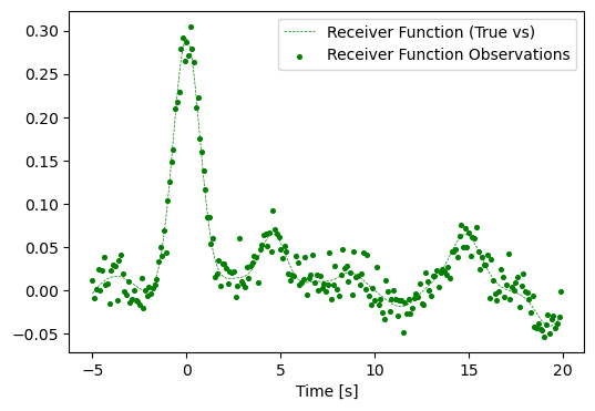
Receiver function

T_SHIFT = 5
T_DURATION = 25
T_SAMPLING_INTERVAL = 0.1
GAUSS = 1
RAY_PARAM_S_KM = 0.07
RF_STD = 0.015

def forward_rf(state):
    voronoi = state["voronoi"]
    voronoi_sites = voronoi["discretization"]
    thickness = Voronoi1D.compute_cell_extents(voronoi_sites)
    vs = voronoi["vs"]
    return pyhk.rfcalc(
        ps=0, 
        thik=thickness, 
        beta=vs, 
        kapa=np.ones((len(vs),))*VP_VS,
        p=RAY_PARAM_S_KM, 
        duration=T_DURATION, 
        dt=T_SAMPLING_INTERVAL, 
        shft=T_SHIFT, 
        gauss=GAUSS
    )

rf = pyhk.rfcalc(
    ps=0, 
    thik=THICKNESS, 
    beta=VS, 
    kapa=np.ones((len(VS),))*VP_VS,
    p=RAY_PARAM_S_KM, 
    duration=T_DURATION, 
    dt=T_SAMPLING_INTERVAL, 
    shft=T_SHIFT, 
    gauss=GAUSS
)
rf_obs = rf + np.random.normal(0, RF_STD, rf.size)

RF_TIMES = np.arange(len(rf_obs)) * T_SAMPLING_INTERVAL - T_SHIFT

_, ax = plt.subplots(figsize=(6, 4))

ax.plot(RF_TIMES, rf, 'g--', label="Receiver Function (True vs)", lw=0.5)
ax.scatter(RF_TIMES, rf_obs, label="Receiver Function Observations", s=7, c="g")
ax.set_xlabel("Time [s]")
ax.legend()

<matplotlib.legend.Legend at 0x7fc03a5c3dc0>

Sample with BayesBay

target_rayleigh = bb.likelihood.Target("rayleigh", 
                            rayleigh_obs, 
                            std_min=0.001, 
                            std_max=0.1, 
                            std_perturb_std=0.002)
target_love = bb.likelihood.Target("love", 
                        love_obs, 
                        std_min=0.001, 
                        std_max=0.1, 
                        std_perturb_std=0.002)
target_rf = bb.likelihood.Target("rf", 
                      rf_obs, 
                      std_min=0.001, 
                      std_max=0.1, 
                      std_perturb_std=0.002)

targets = [target_rayleigh, target_love, target_rf]
fwd_functions = [forward_rayleigh, forward_love, forward_rf]

log_likelihood = bb.likelihood.LogLikelihood(targets, fwd_functions)

inversion = bb.BayesianInversion(
    parameterization=parameterization, 
    log_likelihood=log_likelihood,
    n_chains=24
)
inversion.run(
    sampler=bb.samplers.SimulatedAnnealing(temperature_start=3), 
    n_iterations=600_000, 
    burnin_iterations=150_000, 
    save_every=150,
    verbose=False
)

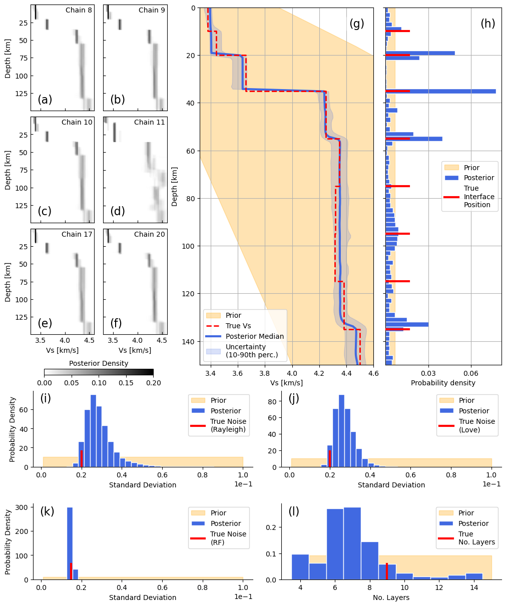
Plot results

results = inversion.get_results(concatenate_chains=True)


sampled_voronoi_nuclei = results["voronoi.discretization"]
sampled_thickness = [Voronoi1D.compute_cell_extents(n) for n in sampled_voronoi_nuclei]
sampled_vs = results["voronoi.vs"]
interp_depths = np.linspace(0, 160, 160)
statistics_vs = Voronoi1D.get_tessellation_statistics(
    sampled_thickness, sampled_vs, interp_depths, input_type="extents"
)

fig = plt.figure(figsize=(10, 12), constrained_layout=True)

gs_main = gridspec.GridSpec(2, 1, figure=fig, height_ratios=[1.8, 1], hspace=0.3)
gs_top = gridspec.GridSpecFromSubplotSpec(
    1, 2, subplot_spec=gs_main[0], width_ratios=[1, 2], wspace=0.8
)


# 6 RANDOMLY CHOSEN CHAINS
# gs_left = gridspec.GridSpecFromSubplotSpec(3, 2, subplot_spec=gs_top[0], wspace=0.001, hspace=0.02)
gs_left = gridspec.GridSpecFromSubplotSpec(
    4, 2, subplot_spec=gs_top[0], wspace=0, hspace=0.04, height_ratios=[1, 1, 1, 0.075]
)

random_chains = np.sort(np.random.choice(np.arange(20), 6, replace=False))
for ipanel, ichain in zip(range(6), random_chains):
    istart = 3000 * ichain  # 600_000 iterations, 150_000 burnin, 24 chains
    iend = istart + 3000
    samples_thickness = sampled_thickness[istart:iend]
    samples_vs = sampled_vs[istart:iend]

    ax = fig.add_subplot(gs_left[ipanel])
    # Your plotting commands for these subplots here
    # Voronoi1D.plot_tessellations(samples_thickness,
    #                               samples_vs,
    #                               input_type='extents',
    #                               ax=ax,
    #                               linewidth=0.1,
    #                               color="k",
    #                               bounds=(0, 150))
    density, Y, X = Voronoi1D.get_tessellation_density(
        samples_thickness, samples_vs, input_type="extents"
    )
    img = ax.pcolormesh(X, Y, density, cmap="binary", vmin=0, vmax=0.2)
    ax.invert_yaxis()
    ax.text(
        x=0.97,
        y=0.98,
        s=f"Chain {ichain+1}",
        va="top",
        ha="right",
        transform=ax.transAxes,
        bbox=dict(facecolor="w", edgecolor="w", alpha=1, boxstyle="square,pad=0.05"),
    )
    ax.tick_params(direction="in")
    # ax.grid()
    row, col = divmod(ipanel, 2)
    if col == 1:
        ax.tick_params(labelleft=False)
    else:
        ax.set_ylabel("Depth [km]")
    if row < 2:
        ax.tick_params(labelbottom=False)
        ax.set_xlabel("")
    else:
        ax.set_xlabel("Vs [km/s]")
    ax.yaxis.set_major_locator(MaxNLocator(prune="both", nbins=7))
    ax.xaxis.set_major_locator(AutoLocator())
    ax.set_xlim(3.3, 4.6)
    ax.text(
        x=0.1,
        y=0.05,
        s=f"({string.ascii_lowercase[ipanel]})",
        va="bottom",
        ha="left",
        fontsize=16,
        bbox=dict(facecolor="w", edgecolor="w", alpha=1, boxstyle="round,pad=0.2"),
        transform=ax.transAxes,
    )

cbar_ax = fig.add_subplot(gs_left[-1, :])
# cbar = fig.colorbar(img, cax=cbar_ax, orientation='horizontal')
# cbar.ax.xaxis.set_label_position('top')  # Move the label to the top
# cbar.set_label('Posterior Density', labelpad=5)
cbar_ax.set_axis_off()
inset_cbar_ax = cbar_ax.inset_axes([0.1, 0.2, 0.8, 0.75])
cbar = fig.colorbar(img, cax=inset_cbar_ax, orientation="horizontal")
cbar.ax.xaxis.set_label_position("top")  # Move the label to the top
cbar.set_label("Posterior Density", labelpad=5)
# INFERRED MODEL AND INTERFACES
gs_right = gridspec.GridSpecFromSubplotSpec(
    1, 2, subplot_spec=gs_top[1], width_ratios=[1.5, 1], wspace=0
)

ax1 = fig.add_subplot(gs_right[0])
ax1.fill_betweenx(
    depth_prior, vmin_prior, vmax_prior, color="orange", alpha=0.3, label="Prior"
)
ax1.plot(
    statistics_vs["median"], interp_depths, "royalblue", lw=3, label="Posterior Median"
)
Voronoi1D.plot_tessellation(
    THICKNESS,
    VS,
    ax=ax1,
    color="r",
    ls="--",
    lw=2,
    label="True Vs",
    input_type="extents",
)

ax1.fill_betweenx(
    interp_depths,
    *statistics_vs["percentiles"],
    color="#4169E133",
    # alpha=0.2,
    label="Uncertainty\n(10-90th perc.)",
)
handles, labels = ax1.get_legend_handles_labels()
handles = [handles[0], handles[2], handles[1], handles[3]]
labels = [labels[0], labels[2], labels[1], labels[3]]

ax1.set_xlabel("Vs [km/s]")
ax1.set_ylabel("Depth [km]")
ax1.grid()
ax1.legend(handles, labels, loc="lower left")
ax1.set_xlim(3.32, 4.6)
ax1.set_ylim(150, 0)
ax1.text(
    x=0.95,
    y=0.97,
    s="(g)",
    va="top",
    ha="right",
    fontsize=16,
    bbox=dict(facecolor="w", edgecolor="w", alpha=0.5, boxstyle="round,pad=0.2"),
    transform=ax1.transAxes,
)

ax2 = fig.add_subplot(gs_right[1])
ax2.fill_between([0, 1 / (150)], y1=0, y2=150, alpha=0.3, color="orange", label="Prior")

ax2 = Voronoi1D.plot_interface_hist(
    sampled_voronoi_nuclei,
    ax=ax2,
    swap_xy_axes=True,
    bins=75,
    fc="royalblue",
    ec="w",
    label="Posterior",
)

for interface_depth in np.cumsum(THICKNESS)[:-2]:
    ax2.axhline(y=interface_depth, xmax=0.2, color="r", lw=3, alpha=1, zorder=5, ls="-")
ax2.axhline(
    y=np.cumsum(THICKNESS)[-1],
    xmax=0.2,
    color="r",
    lw=3,
    alpha=1,
    zorder=5,
    ls="-",
    label="True\nInterface\nPosition",
)

handles, labels = ax2.get_legend_handles_labels()
handles = [handles[0], handles[2], handles[1]]
labels = [labels[0], labels[2], labels[1]]

ax2.tick_params(labelleft=False)
ax2.set_ylabel("")
ax2.set_ylim(*ax1.get_ylim())
ax2.grid()
ax2.legend(handles, labels, loc="center right")
ax2.xaxis.set_major_locator(MaxNLocator(prune="both", nbins=3))
ax2.text(
    x=0.95,
    y=0.97,
    s="(h)",
    va="top",
    ha="right",
    fontsize=16,
    bbox=dict(facecolor="w", edgecolor="w", alpha=0.5, boxstyle="round,pad=0.2"),
    transform=ax2.transAxes,
)


# NOISE STD
gs_bottom = gridspec.GridSpecFromSubplotSpec(
    2, 2, subplot_spec=gs_main[1], wspace=0.05, hspace=0.05
)

std_min_sw, std_max_sw = 0.001, 0.1
std_min_rf, std_max_rf = 0.001, 0.1

# Rayleigh
ax3 = fig.add_subplot(gs_bottom[0])
ax3.fill_between(
    [std_min_sw, std_max_sw],
    1 / (std_max_sw - std_min_sw),
    alpha=0.3,
    color="orange",
    label="Prior",
)
pdf, bins, _ = ax3.hist(
    results["rayleigh.std"],
    density=True,
    bins=np.linspace(std_min_sw, std_max_sw, 35),
    fc="royalblue",
    ec="w",
    label="Posterior",
)
ax3.axvline(
    x=RAYLEIGH_STD, ymax=0.2, color="r", lw=3, alpha=1, label="True Noise\n(Rayleigh)"
)
ax3.ticklabel_format(style="sci", axis="x", scilimits=(0, 0))
ax3.legend(loc="upper right")


ax4 = fig.add_subplot(gs_bottom[1])
ax4.fill_between(
    [std_min_sw, std_max_sw],
    1 / (std_max_sw - std_min_sw),
    alpha=0.3,
    color="orange",
    label="Prior",
)
pdf, bins, _ = ax4.hist(
    results["love.std"],
    density=True,
    bins=np.linspace(std_min_sw, std_max_sw, 35),
    fc="royalblue",
    ec="w",
    label="Posterior",
)
ax4.axvline(x=LOVE_STD, ymax=0.2, color="r", lw=3, alpha=1, label="True Noise\n(Love)")
ax4.ticklabel_format(style="sci", axis="x", scilimits=(0, 0))
ax4.legend(loc="upper right")


ax5 = fig.add_subplot(gs_bottom[2])
ax5.fill_between(
    [std_min_rf, std_max_rf],
    1 / (std_max_rf - std_min_rf),
    alpha=0.3,
    color="orange",
    label="Prior",
)
pdf, bins, _ = ax5.hist(
    results["rf.std"],
    density=True,
    bins=np.linspace(std_min_rf, std_max_rf, 35),
    fc="royalblue",
    ec="w",
    label="Posterior",
)
ax5.axvline(x=RF_STD, ymax=0.2, color="r", lw=3, alpha=1, label="True Noise\n(RF)")
ax5.ticklabel_format(style="sci", axis="x", scilimits=(0, 0))
ax5.legend(loc="upper right")

ax6 = fig.add_subplot(gs_bottom[3])
ndim_min, ndim_max = 4, 15
ax6.fill_between(
    [ndim_min, ndim_max],
    1 / (ndim_max - ndim_min),
    alpha=0.3,
    color="orange",
    label="Prior",
)

ax6.hist(
    results["voronoi.n_dimensions"],
    bins=np.arange(ndim_min - 0.5, ndim_max + 0.5),
    fc="royalblue",
    density=True,
    ec="w",
    label="Posterior",
)
ax6.axvline(
    x=9, ymax=0.2, color="r", lw=3, alpha=1, label="True\nNo. Layers", zorder=100
)
ax6.legend()

for ipanel, ax in enumerate([ax3, ax4, ax5, ax6]):
    if ipanel == 0 or ipanel == 2:
        ax.set_ylabel("Probability Density")
    ax.set_xlabel("Standard Deviation")
    ax.spines["right"].set_visible(False)
    ax.spines["top"].set_visible(False)
    ax.text(
        x=0.03,
        y=0.97,
        s=f"({string.ascii_lowercase[8 + ipanel]})",
        va="top",
        ha="left",
        fontsize=16,
        bbox=dict(facecolor="w", edgecolor="w", alpha=0.5, boxstyle="round,pad=0.2"),
        transform=ax.transAxes,
    )

ax6.set_xlabel("No. Layers")
# ax6.legend()

plt.show()

results.keys()

dict_keys(['voronoi.n_dimensions', 'voronoi.discretization', 'voronoi.vs', 'rayleigh.std', 'love.std', 'rf.std', 'rayleigh.dpred', 'love.dpred', 'rf.dpred'])